4. Design tab

4.1 Principles

The Design tab prepares a four-axis cut from two paths: the side 1 path (in blue) and the side 2 path (in red). The software makes no assumption about the part: a wing, a fuselage, a letter or any other object is handled the same way.

In this manual, a path is a sequence of segments joining points; a project is the full set of parameters of a cut (the two paths, the spacing, the block, the margins, the cutting settings). The word profile is reserved for wing profiles.

A few rules apply everywhere in this tab:

• Everything that is added (a spar, a shape, an intermediate profile) becomes a sequence of points like any other. Any point can then be moved, deleted or added.
• For a project to be cut, the two paths must have the same number of points. The wire passes through the points with the same number on both sides at the same time.
• Every action is recorded: Undo and Redo in the toolbar (or Ctrl+Z / Ctrl+Y) go back up to 40 states. Each document has its own history. Undo changes neither the material nor the settings of the Cutting tab.
• The axes: X is the horizontal axis (the chord), Y the vertical axis (the thickness), Z the axis running from one side to the other (the spacing).

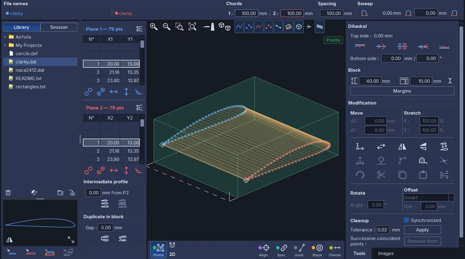
When an empty project opens, a welcome card appears in the middle of the 3D view. It offers Load the example (the supplied NACA 2412 profile), Open a project…, Recent files and Empty project. It disappears as soon as a path is imported; the cross hides it for the session, and a setting stops it from being shown again.

4.2 Importing a path or a project

4.2.1 The library

The left column shows the library, the same one as in the Wing, Sections and Views tabs (each with its own import buttons). Two buttons at the top choose its source: Library, the Library folder of the data folder (by default Documents/HotWire4X/Library), and Session, the profiles of the open project (see below). The Library folder is the recommended place for all profile and project files: they are then visible at a glance and ready to use.

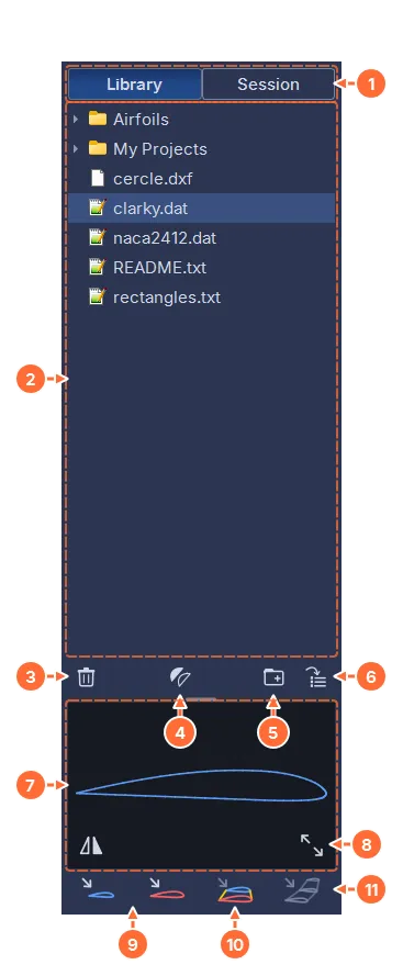
1. Library and Session: the source of the list.
2. The file tree. Clicking a file shows it in the viewer; a folder expands. A file or a folder is moved by dragging it onto another folder, and renamed with F2 or a double-click.
3. Move the selected file to the recycle bin, after confirmation (it can still be recovered from the system’s recycle bin).
4. Open the image vectorization tool (see chapter 13).
5. Create a folder.
6. Import an external file into the library (a copy is made).
7. The viewer: the selected file is drawn. When it holds several paths, each has its own color; a project also shows its block.
8. Mirror the preview (DAT, COR, DXF and SVG files), and enlarge the viewer: the file tree moves to the left, the preview to the right, and the 3D view and the right column are hidden; a second click restores the layout.
9. Import profile into Plane 1 and Import profile into Plane 2: the selected path goes into side 1 or side 2.
10. Import document: adds the selected document of a project file as a new document of the workspace.
11. Open the full project: replaces the workspace with the selected file.

The supported formats are described in chapter 14: DAT and COR profiles, DXF, SVG, TXT; HotWire4X .hw4x and FilChaudNX .fnx projects.

4.2.2 Session profiles

The Session button replaces the file tree with the list of profiles that the open project already contains, sorted by tab and then by element. It lets you reuse in one tab a profile drawn in another, without going through an export:

• Design: each document that has at least two points on one side, with its sides (only one when the two are identical);
• Views: the side view and the top view of each element, as a closed outline, as the Views tab exports it;
• Wing: the ribs as they are drawn, numbered R1, R2… from the inner rib of the wing;
• Sections: the outer and inner outlines of both faces of each segment (for example “T1 · Left · Outer”).

The list is read again each time it is shown; an empty project shows “No profile”. The viewer, the mirror and the Import profile into Plane 1 and Import profile into Plane 2 buttons work as for a file. The import copies the points, without their selections: no synchronization point is carried over. Import document and Open the full project stay inactive: a session document is duplicated from its chip’s menu (chapter 3).

4.2.3 Single-path file

Select the file, then click Import profile into Plane 1. The first time, the path is automatically copied into side 2: a wing profile imported only once gives a rectangular panel ready to be adjusted.

To have a different path on the other side, select the other file and click Import profile into Plane 2. The existing path is replaced (the operation can be undone with Undo).

A DAT or COR profile contains no dimensions: it takes the chord of the side it is imported into (the value shown in the banner), or 100 mm on an empty side. Replacing the profile of a wing that is already at its dimensions therefore keeps its chord; after a first import, on the other hand, the real chord must be entered (see the banner, below). DXF, SVG and TXT files are in millimeters and keep their size.

4.2.4 Multi-path file: the selection window

When the file contains several paths (a DXF with several outlines, a TXT file, an alphabet, a project with two sides), the Select Trajectories window opens.

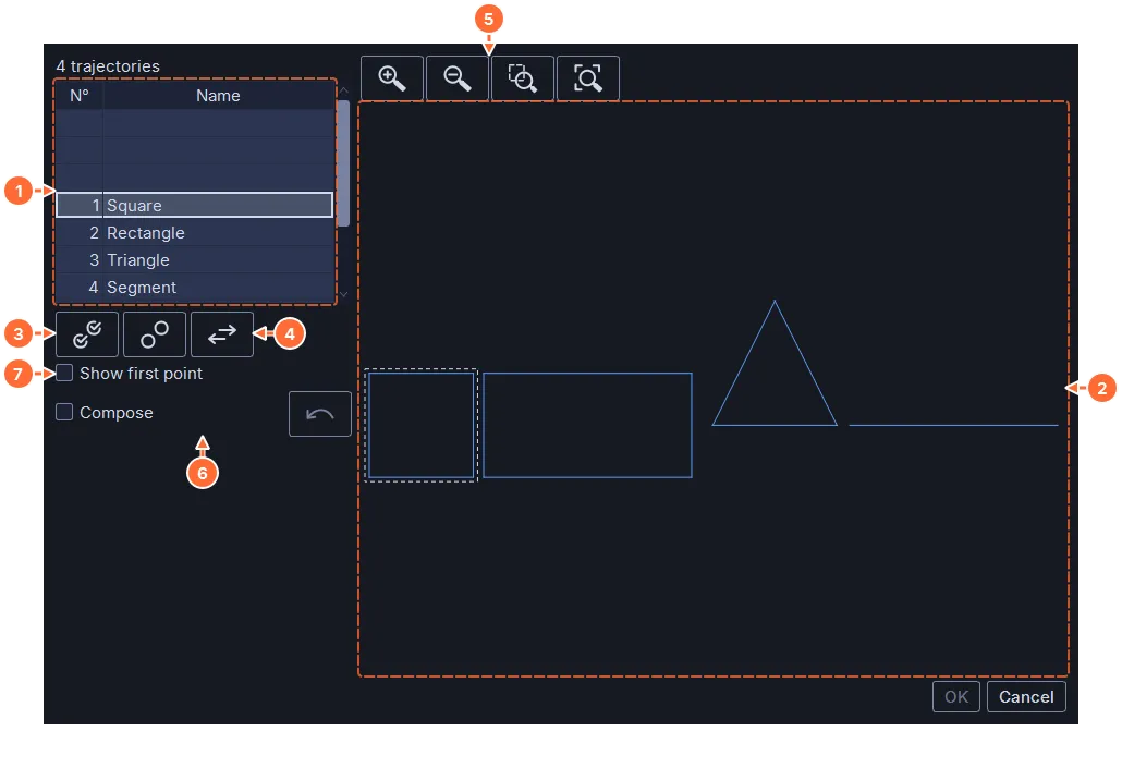
1. The path counter: the current row is highlighted in the preview. The scroll bar steps from one path to the next, which is invaluable when paths overlap or are too small to be clicked.
2. The preview: clicking a path selects it and moves the counter.
3. Select All and Deselect All.
4. Reverse reverses the point order of the paths in the window (check Show first point to see the effect).
5. The zoom buttons, as in the 3D view.
6. The Compose box: in compose mode, the paths clicked one after another are chained into a single path. This is how a word is written from an alphabet file: check Compose, then click the letters in order. The undo button removes the last letter.
7. Show first point highlights the first point of each path and its direction of travel.

OK imports the selection. Several paths selected without Compose are chained in the order of selection.

4.2.5 Full project, several documents

A .hw4x file can contain several documents (the working document, free documents, panels transferred from the Wing tab, Sections sheets, views). When it does, a Document list appears above the viewer to choose which one to show.

• Import profile into Plane 1 or Import profile into Plane 2 takes one side of the chosen document: the selection window opens when the document has two different sides; a document whose two sides are identical offers only one.
• Import document adds the chosen document as a free document of the current workspace.
• Open the full project opens the whole file, like File ▸ Open project.

A FilChaudNX .fnx project opens the same way: the two paths, the spacing and the block are carried over; the selections and the cutting settings have to be redone.

4.2.6 Files outside the library

The File menu offers Import profile ▸ Import profile to Plane 1… or Import profile to Plane 2…, and Open project…, to fetch a file from anywhere on the computer. Import documents… adds all the documents of another .hw4x file to the current workspace.

4.2.7 Saving

As soon as a project is started, save it with File ▸ Save or Ctrl+S. The first time, a .hw4x file name is requested; after that, the name appears in the window title and an asterisk flags unsaved changes. Save As… creates a copy under another name.

The .hw4x file contains the whole workspace: all the documents (with their material and their background images), the wings, the segments, the views, the assembly and the reference images. The state of the Cutting tab’s mirror is not saved (it depends on the day’s cut).

4.3 The banner: file names, chords, spacing, sweep

1. File names: the source file of each side (blue dot for side 1, red for side 2). For a panel transferred from the Wing tab, the origin follows the names (“From wing panel 3”).
2. Chords: the horizontal dimension (in X) of each path, measured on the profile points (see Chords mode). Changing the value scales the path uniformly: the height follows in proportion. This is the first thing to check after the first import of a DAT.
3. Spacing: the distance between the two sides, that is, the length of the panel for a wing. Tip: keeping a small spacing while working on the paths makes the 3D view easier to read; enter the final value just before cutting.
4. Sweep: the horizontal offset of one side relative to the other. Only the value at the leading edge (on the right, Xmax) can be edited; the value at the trailing edge is recalculated. The three buttons Min, Center and Max align the trailing edges, the midpoints or the leading edges.

All numeric values are written with two decimals, and a comma is accepted as well as a point. A value is applied when you leave the field or press Enter or Tab. The ↑ and ↓ arrow keys change the value by one step, Ctrl + ↑ / ↓ by ten steps, Shift + ↑ / ↓ by a tenth of a step (Page Up / Page Down by ten steps); in this tab, a value set this way is applied with Enter, and the field keeps the focus: you can go on changing it. The mouse wheel never changes a field.

Changes to the chord, the sweep and the dihedral apply to the profile points. Points that are not part of it (a spar, a leading-edge exit, a junction path, see Chords mode) are moved as a unit with their attachment point, without being resized: an 8 mm spar hole stays an 8 mm hole when the chord changes.

4.4 The point lists

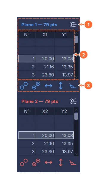
1. The header gives the side and the number of points. The button on the right closes the path: it adds a last point identical to the first.
2. The table: the point number and its X and Y coordinates in millimeters. The framed middle row is the current point; in the 3D view it is marked by a white diamond. The list scrolls with the bar, the mouse wheel, or the keyboard once the list has been clicked: ↑ and ↓ (one point), Page Up / Page Down (four points), Home / End. Clicking a row selects the point without scrolling the list, following the mode’s rule: in Points mode, this point alone; in a marking mode, it toggles (Ctrl and Shift: see The gestures); a double-click opens its coordinates. The numbers of the two points of a null segment (two successive coincident points) are written in red (see The cleanup tool).
3. The five automatic selection buttons (see below).

The first point of a path is number 1. In the 3D view, a thick arrow starts from the first point in the direction of travel. Clicking a point in the 3D view selects it (in Points mode, this point alone) and moves the list to that point (see Selecting points).

For a wing, it is important to close the paths: a profile with an open trailing edge gives a trailing edge with no clean edge. The close button in the header creates the closing point; Undo takes you back.

4.4.1 Entering a point’s coordinates

A double-click on a point of the 3D view (the one nearest the cursor), on a marker of the magnifier or on a row of a list opens the Point coordinates window, in every selection mode; right-click opens it too. From the 3D view, the list first moves to that point; from a list, the rows do not move. The selection stays as it was before the double-click: the first click, which had changed it, is taken back. A right-click drag is still a pan of the view. With the 2D button, the point with the same number on the other side moves by the same offset.

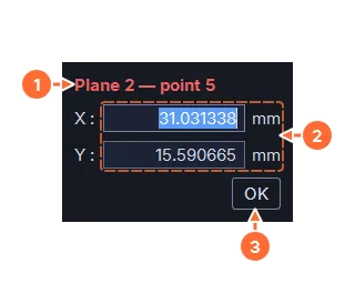
1. The side, in its color, and the point number.
2. X and Y in millimeters, at full precision: up to six decimals, those of the source file, whereas the lists round to two.
3. OK applies.

Enter or Tab moves from X to Y, then to OK; Enter on OK applies; Esc closes without touching the point. A field left as it is keeps the point’s exact value; a typed value is written as typed. The change counts as one undo step. If the edited point becomes the lowest point of the profile, the project is realigned on the vertical position of the block, as after a move.

4.5 Dihedral and alignments

The Dihedral frame in the right column sets the vertical position of one side relative to the other.

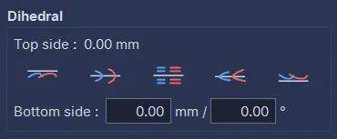
• Top side (read-only): the vertical gap between the highest points of the two sides.
• The five buttons align the two sides: Top (the upper surfaces), Xmax (the leading edges), Center (the midpoints), Xmin (the trailing edges), Bottom (the lower surfaces).
• Bottom side, in mm and in degrees: the vertical gap between the lowest points of the two sides, and the same gap expressed as an angle from the spacing; changing one updates the other. For a wing, this is the shim to slip under side 1. Positive when side 1 is higher.

The gaps are measured on the profile points (see Chords mode). Changing the dihedral moves side 1; side 2 does not move.

4.5.1 Aligning on a real or virtual point

The Align. selection mode (see below) aligns the two sides on the centroid of chosen points: the center of a circle, a vertex, the midpoint of a segment. Select one or more points on each side; the centroid of each selection appears in the 3D view, drawn as a target (a circle and a cross, in its side’s centroid color, over the points). Click Align on centroid: side 1 is moved so that the two centroids coincide. This is the tool for fuselages built from sections.

4.6 The block

The Block frame describes the raw block of material. Its dimensions are derived from the project and the margins; only the margins, the thickness and the vertical position can be set.

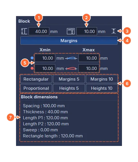
1. The thickness of the block (vertical dimension, in Y).
2. The vertical position: the distance between the underside of the block and the lowest point of the cut. It is used to optimize the machine’s travel.
3. The dimensions button: it shows in the 3D view, for each side and in its color, the vertical dimensions between the extreme points of the profile (the lowest, the highest, the leftmost, the rightmost) and the bottom and top faces of the block. It is released at startup.
4. Margins expands the rest of the frame.
5. The four margins, on the left (Xmin) and on the right (Xmax) of each side.
6. The automatic settings: Rectangular fills in the sweep to get a rectangular block; Margins 5 and Margins 10 set the four margins to 5 or 10 mm; Proportional scales the margins of the smaller side by the ratio of the chords; Heights 5 and Heights 10 set the thickness with 5 or 10 mm of margin above and below.
7. Block dimensions (read-only): spacing, thickness, length of each side, sweep, length of the bounding rectangle.

To use a block whose dimensions are already known, adjust the margins until those dimensions are reached. Since the block depends on the project, check it one last time just before cutting; the Cutting tab’s Blocks summary shows how to cut each block from a sheet of material, with all its dimensions (chapter 5).

4.7 The 3D view

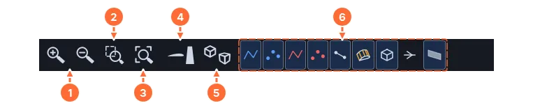
1. Zoom + and Zoom -.
2. Zoom by selection: click the button (or press the Z key), then draw a rectangle in the view.
3. View all: fits what is displayed into the window.
4. The view button goes from the side view to the top view, then to the front view, then back to the side view; from a 3D view, it goes to the side view. The side view looks from side 2, with side 1 behind; the top view puts side 1 at the top of the screen; the front view looks from the leading edge (Xmax), with side 1 on the right: it shows the dihedral of a panel, for example against a Front view background image (see below).
5. 3D Ortho / 3D Perspective; from a side, top or front view, the button switches to 3D ortho.
6. The nine display toggles, one button per element: side 1 segments, side 1 points, side 2 segments, side 2 points, the wire, the envelope (the surface between the two sides), the block, the direction markers (a chevron in the middle of each segment, hidden at first because they clutter the view), the background images. The wire and the envelope are grayed out as long as the two paths do not have the same number of points. Releasing the points button of a side disables that side (see Disabling a side).

The wire joins the current point of each list. Scrolling a list slides the wire along: it is a first simulation, before the one in the Cutting tab.

In every selection mode, junction segments are drawn dashed, and each stop point is circled by a pink ring, the same as in the Cutting tab.

Coincident points are flagged too, in every mode: a red ring on each null segment (two successive points at the same place, within the cleanup tolerance), and a “×2”, “×3”… badge, in the color of its side, where several points of the same side overlap, for example the closing point of a closed profile, or the way in and the way back of a slot. Where selected and unselected points are drawn at the same place, a half-filled ring, in the mode’s color, signals that the selected point hides another one that is not selected. A click on coincident points opens the magnifier (see Selecting points). The status bar adds the number of null segments on each side (”⚠ 1 null segment(s) on P1”). Null segments are removed with Remove them (see The cleanup tool).

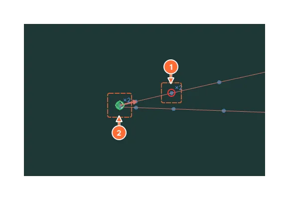
1. A null segment: the red ring, and the “×2” badge of the two coincident points.
2. The closing point of a closed profile: its “×2” badge, and the half-filled ring, because only point #1 is selected, not the closing point.

Hovering over a point surrounds it with a thin circle, and a label near the cursor gives its side, its number and its coordinates (“P1 #12 (120.00 ; 8.50)”); over coincident points, it gives the numbers on each side with their state (“P1 #1, #41 ✓ · P2 #1 — 3 points, 1 selected”). The circle and the label can be turned off, and the opacity of the label’s background adjusted, in the settings, Mouse page (chapter 3).

With the mouse:

• mouse wheel: zoom around the cursor;
• right button: pan the view;
• double-click on a point, or right-click without dragging: enter its coordinates (see The point lists);
• middle button, or Alt + left-button drag: rotate the view (in side, top and front views, this gesture pans the view);
• left button: select (see below); Alt + click: the magnifier.

4.8 Selecting points

4.8.1 The six modes

Under the 3D view, six buttons choose the selection mode. Each mode has its own selection and its own color; a point can be selected in one mode and not in another. The active mode is shown at the top right of the 3D view and in the status bar. Changing mode brings the right column back to its Tools page.

The Points mode, on the left, is for editing the drawing: a click there takes a single point, as in the 2D editors of the Sections and Views tabs. The five marking modes, on the right, mark points for a specific purpose (the synchronization anchors, the junctions, the stops…): their selection is data, and a click there toggles the point without touching the other marks.

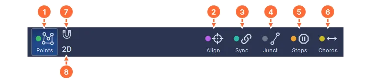
1. Points: the working mode. Move, add, delete, transform points; all the modification tools relate to it.
2. Align.: align the two sides on a centroid (see Dihedral and alignments).
3. Sync.: choose the synchronization points (see Synchronization).
4. Junct.: mark the junction segments, traveled without wire offset (see the modification tools).
5. Stops: place the stop points of the cut (see Stop points).
6. Chords: define the points that are part of the profile (see the next section).
7. The Snap magnet, in Points mode only (see Moving points with the mouse); hidden in the other modes, it keeps its place.
8. The 2D button, in every mode: the two sides are selected together (see Working in 2D).

4.8.2 The gestures

A click always targets the point nearest the cursor, and moves the list to that point. In Points mode (the same gestures as in the 2D editors, chapters 9 and 10):

• Click on a point: it becomes the only selected point. This way you go from one point to another without deselecting.
• Ctrl + click: adds the point to the selection, or removes it, without touching the others (the cursor shows ±).
• Shift + click: adds the range along the path, from the current point of the list (the hollow diamond) to the clicked point, which becomes the current point (over a point, the cursor shows +++).
• Ctrl + Shift + click: removes that range (over a point, the cursor shows −−−).
• Box (left button and drag starting from empty space): replaces the selection with the points inside the box, on the sides whose points are displayed; Shift + box adds them (away from a point, the cursor shows a + on the corner of a rectangle, then a plain + while the box is drawn), Ctrl + box removes them.
• Click on empty space: deselects everything, on the sides whose points are displayed. So does Esc.

In the marking modes:

• Click on a point: toggles its mark (marked if it was not, unmarked otherwise); the other marks stay.
• Ctrl + click: unmarks the point, never marking it (the cursor shows a −).
• Shift + click and Ctrl + Shift + click: mark or unmark a range, as in Points mode.
• Box: marks the points inside the box; Ctrl + box unmarks them.
• Click on empty space: changes nothing, so that marks are not lost by accident. It is Esc that unmarks everything.

Everywhere:

• Double-click on a point: the Point coordinates window (see The point lists), the selection staying as it was before the double-click; right-click opens it too.
• Alt + click: opens the magnifier on this point (see The magnifier).
• The cursor changes as soon as Ctrl or Shift is pressed, without moving the mouse.

In a list, a click on a row follows the same rules for that single number, according to the mode (click, Ctrl + click, Shift + click and Ctrl + Shift + click from the middle row); in Points mode, a plain click also deselects the other side. The rows do not move.

With the keyboard:

• Esc first closes the magnifier or leaves the measuring tool if it is armed, otherwise deselects everything in the current mode; Ctrl + A selects everything. Both act on the sides whose points are displayed (on both sides with the 2D button).
• Delete or Backspace: deletes the selected points, in Points mode only, like the Delete selected points button when it is active.

Under each list, five buttons: Unselect all, Select all, Select Xmin Xmax (the leftmost and the rightmost point), Select Ymin Ymax (the lowest and the highest), Selection >30° (all the vertices with an angle of more than 30 degrees). They act only on their own side (on both with the 2D button).

Selected points take the mode’s color, in the 3D view and in the lists. The status bar gives the number of selected points on each side; in Points mode, as soon as at least two points are selected on a side, it adds the X and Y extent of the selection (“P1: 4 sel. 20.26 × 10.00 mm”). The mouse button, on the left of the status bar, sums all this up (chapter 3).

4.8.3 The magnifier

Points drawn at the same place on the screen cannot be told apart with a click: the closing point of a closed profile, the way in and the way back of a slot, or side 1 drawn over side 2 in side view. A click on such points selects nothing: it opens the magnifier, centered on the targeted point. Alt + click opens it on demand on any point.

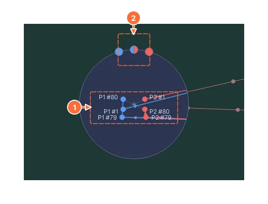
1. The coincident points, spread apart: side 1 on the left, side 2 on the right, each with its number, its state (the mode’s color if it is selected) and its two segments in their real direction, with an arrowhead in the direction of the path. A null segment is drawn in red, a junction dashed; a small cross marks the place of the click.
2. The dots on the top of the disc take every point shown by the magnifier: blue = side 1, red = side 2, blue and red = both sides. In Points mode, a click on a dot takes these points alone; in a marking mode, it marks them all if one was missing, and unmarks them all otherwise.

In the magnifier:

• a click on a marker follows the mode’s rule, as in the view (in Points mode, this point alone; Ctrl adds or removes it; Shift adds the range); keys 1 to 9 take the markers in order;
• a double-click or a right-click on a marker opens its coordinates;
• the mouse wheel enlarges or reduces, from ×3 to ×16;
• hovering over a marker lights it up in the 3D view, with its segments;
• beyond 8 coincident points, or 12 points in all, the magnifier becomes a list, scrolled with the mouse wheel; the dots then take the whole list.

The magnifier stays open during clicks, to take several points (Ctrl + click in Points mode). Esc, a click outside it or a movement of the view closes it. The measuring tool also opens it on an ambiguous click.

4.8.4 Working in 2D

The 2D button, under the magnet, links point #i of side 1 to point #i of side 2, in every mode, every view and both lists. Each gesture selects both points, the lists scroll together, Esc and Ctrl + A take both sides, a drag or a typed coordinate moves both points by the same offset, and closing a path closes both. Each tool therefore edits both sides the same way: two identical sides stay identical, whatever the view; two synchronized but different sides, such as those of a tapered wing, are edited as a pair. The status bar shows “Modification (2D)”, and a 2D label appears to the left of the mode label, at the top right of the 3D view.

• The button needs the same number of points on both sides; otherwise it is grayed out, and its tooltip gives the two numbers.
• Turning it on merges the selections of the two sides, in each mode, and checks the cleanup’s Synchronized box; this is one undo step. Its state is saved with the document.
• It turns on by itself for cuts transferred from the Views tab (chapter 10). A profile imported into an empty project, and copied to both sides, leaves it off.
• It turns off by itself when an operation leaves different numbers of points, or when a profile is imported on one side only; the status bar says so (“2D editing off: P1 has 52 points, P2 50”). Undo goes back.
• Stops mode stays linked, whatever the button.

4.8.5 Disabling a side

To work on one side only, disable the other: release its Points P1 or Points P2 display button, in the 3D view bar. Its points disappear and no longer react (no click, no box, no magnifier), and no modification tool touches it; its selection is kept and comes back with its points. The mirrors, the reversal, the first-point change and the cleanup, which take the whole path when no point is selected, then take only the active side; Copy ignores the disabled side and Paste inserts nothing into it. Swap Plane 1 / Plane 2, Align on centroid, Synchronize and the cleanup’s Synchronized box, which affect both sides, are grayed out as long as a side is disabled. The status bar shows it (“P2 disabled”), and the button’s tooltip says what it does (“Disable P2…” when pressed, “Enable P2…” when released).

With the 2D button, a hidden side stays active: it still follows the other one, so that you can work in 2D with a single side drawn.

4.8.6 Moving points with the mouse

In Points mode, dragging a point moves it: if it was not selected, it becomes the only selected point and moves alone; if it is part of the selection, all the selected points follow it, each in its own plane. Shift + Ctrl + drag moves the selection starting from anywhere. Shift during the drag locks the movement to a single axis, horizontal or vertical. Over a point, the cursor takes the move shape, as with Shift + Ctrl away from a point when points are selected; a drag started from empty space draws a box.

The view does not change during the move. In a 3D view, each point stays in the plane of its side and the grabbed point stays under the cursor. Shift + Ctrl + drag started from empty space follows the plane of the selected points, or the plane halfway between the sides if both sides have some; both sides then receive the same offset. A plane seen almost edge-on moves only in the direction visible on the screen. To place points of one side precisely relative to those of the other, first switch to the side view with the view button.

The Snap magnet (the small button to the right of Points, released at first; its state is remembered) puts the grabbed point exactly on a target: a point of either side, or the origin of a side, as soon as it comes within 12 pixels. In a 3D view, the magnet takes only the targets of the grabbed point’s side: to put a point onto the other side, switch to the side view. The target is circled and the status bar names it (“Snapped onto P2 #34”); the other selected points follow by the same offset. Holding Alt moves freely. The dX and dY fields of Move then refine to the hundredth (see The modification tools).

Coincident points of which only some are selected (the half-filled ring, see The 3D view) still move: only the selected points go, and the status bar names those that stay behind (“P1 #41, coincident, does not follow”), during the drag and after it. A disabled side does not move.

4.9 Paths that leave the block or the profile

When a path leaves the main profile (an X-cut at the leading edge, a spar that opens onto the surface, a junction path to the outside), the chords, the sweep, the dihedral, the heights and the block margins must be computed on the profile alone.

That is what Chords mode is for: the points selected in this mode (in yellow) are those of the profile; the others are ignored by these calculations. All points are selected by default: after an import, in a new document, after a tool that rebuilds the path (synchronization, offset, cleanup). You only need to deselect the points that must not count. A side always keeps chord points: deselecting everything shows a message and selects all the points of the side again.

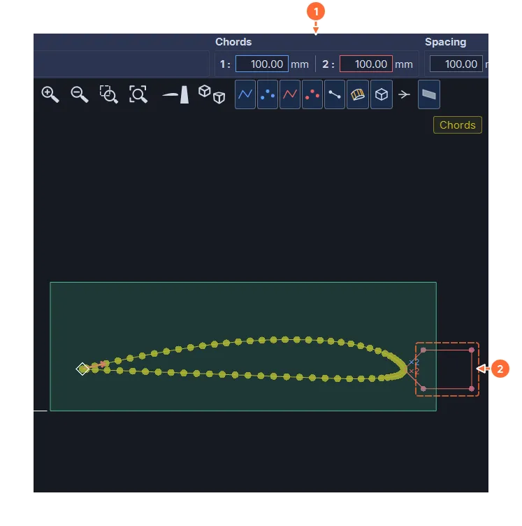
1. The chord shown remains that of the profile alone.
2. The X-cut: its points are not selected in Chords mode.

Points created afterward follow the profile: a point inserted in the middle of a segment, or a closing point, is in the chord when its neighbors are; pasted points, when their anchor point is; a smoothed portion, when it was. An inserted shape (spar, hole, X-cut, free-form shape) is not, but its insertion point and the point that returns onto it stay in: the shape therefore does not change the chords. A panel transferred from the Wing tab arrives with the profile points and the insertion point of each element marked.

4.10 The cleanup tool (very important)

The Cleanup section, at the bottom of the Modification frame (Points mode), deletes double points and “almost” aligned points. The Tolerance (0.02 mm at first, remembered from one session to the next) is the deviation below which a point is considered aligned with its neighbors.

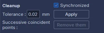
It is very important to clean up the paths before a cut: aligned points serve no purpose, they multiply the segments and can distort the calculation of the wire offset, especially when they are very close together. The Cutting tab also warns you when two consecutive points nearly coincide.

• With no selection, Apply cleans up both whole paths. The Synchronized box removes a point only if its counterpart on the other side can be removed too: the two paths keep the same number of points (see Synchronization).
• With a selection, only runs of at least three selected points are cleaned up, the first and the last point of each run being kept.
• In every case, the markings stay: an alignment, synchronization, junction or stop point is never removed, nor the point kept between two junction points (without it, the stretch between them would become a junction, cut without offset). Each stretch between two such points is cleaned up on its own, and the points that are kept keep all their marks, chords included; only the Points mode selection is cleared.

The Successive coincident points row, under Apply, handles only the null segments, those points that repeat the previous one within the tolerance (an import, a paste, a badly closed slot can leave some). Remove them deletes them without touching the rest of the path, and carries their markings (stop, synchronization, junction, chord) over to the point that is kept. With Synchronized checked and the same number of points on both sides, the points go in pairs, to keep the two paths matched: if this takes away, on the other side, a point that is not a duplicate, a window names it and asks for confirmation. The button is active as soon as a side has a null segment; the operation counts as one undo step.

Apply the cleanup once the paths are at their final dimensions. The cleanup is applied automatically when a DXF or an SVG is imported (these formats produce many useless points); its tolerance is set in the Settings, and the file can be imported again with another value.

4.11 The modification tools

The Modification frame is shown in Points mode. It groups two move fields, two stretch fields, a grid of fifteen tools, rotation, offset and cleanup.

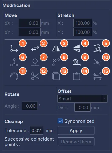
A tool is available or grayed out depending on the selection. The general rule: with no point selected, the mirrors and the direction reversal apply to the whole project; as soon as a point is selected anywhere, only the selection is affected, and a side with no selection is left untouched. Change first point handles each side separately: a side with no selection is renumbered entirely.

4.11.1 With no point selected

• Mirror horizontal (3): symmetry about a vertical axis. Useful after importing a drawing whose X axis is reversed.
• Mirror vertical (4): symmetry about a horizontal axis.
• Reverse path direction (2): when the wire travels the wrong way.
• Swap Plane 1 / Plane 2 (5): swaps the two sides, which mirrors the whole wing. The block margins and the background images of the two sides are swapped with them, as are the end angles of a wing panel cut flat (chapters 5 and 8), which move to the other side with their face. These angles cannot be edited in Design: an import into a side erases them, and only a new transfer from the Wing tab writes them again.
• Change first point (1): the current point of each list (the framed row) becomes point number 1. First move the lists to the new first points. Only the numbers change: the markings (junctions, synchronization, stops, chords) stay on their points, and a closed profile stays closed (its closing point follows the new first point).

4.11.2 Insert shape (spar, hollow, X-cut, free-form shape)

The tool (7) becomes active when a single point is selected on one side, or one on each side: the insertion point. It opens the Insert shape window. The shape is inserted, with the same parameters, on each side that has an insertion point.

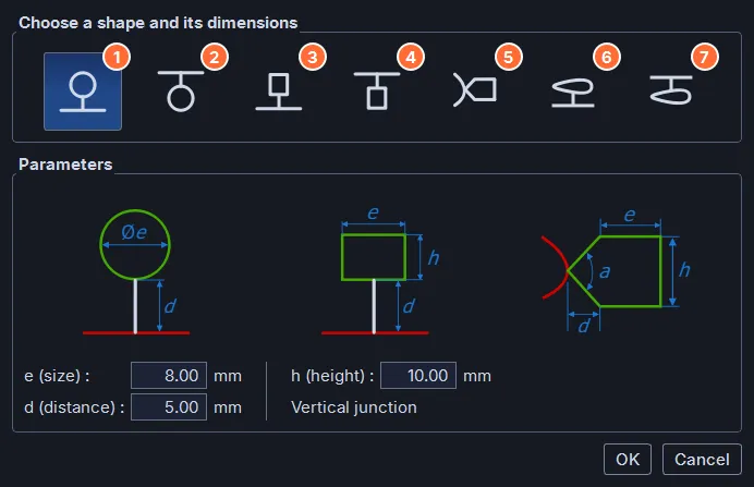
1. A circular hole or spar, entering upward from the insertion point.
2. A circular hole or spar, entering downward.
3. A rectangular hole or spar, entering upward.
4. A rectangular hole or spar, entering downward.
5. An X-cut at the leading edge: it splits the block in two with the best cut quality.
6. A free-form shape, entering from below the insertion point.
7. A free-form shape, entering from above the insertion point.

The parameters, explained by the drawings in the window: e (the diameter or the width), h (the height of a rectangle or of the X-cut), d (the distance between the insertion point and the shape). The arrow keys change these fields like the other numeric fields. Each shape uses only its own parameters; the free-form shapes use only d. For the X-cut, the window shows its angle a, which is not typed in: it follows from h and d (90° with the starting values, e = 8, h = 10 and d = 5 mm) and follows each of their changes. The other shapes enter through a vertical junction: the angle row then reads “Vertical junction”. OK inserts the shape.

The inserted shape is selected automatically: Shift + Ctrl + drag moves it right away. After the shape, the path comes back to the insertion point. For a hole or a spar, the out-and-back run that connects it to the profile is marked as a junction (segments traveled without offset, see below); with d = 0, the spar starts from the insertion point and comes back to it, with no junction path: for a spar that you will move afterward, choose d greater than 0. When the insertion point touches a junction already in place (the return of a shape inserted just before, or the entry of a shape that follows), an unmarked point is added between the two, so that the stretch of profile between them is still cut with its offset. The X-cut has no junction, it is a real cut; its tip is the insertion point itself. The shape is not part of the chords (see Chords mode). For dimensions that differ from one side to the other (tapered spar), insert one side at a time: one point selected on one side only, then on the other, with other parameters.

The two free-form shapes switch the tab to INSERT MODE (a banner says so): the window becomes an independent project in which the shape is drawn with all the usual tools, then a new click on the Insert shape button injects it into the original project, after the insertion point, followed by a return point. Entering from below, the lowest point of the drawing is placed at distance d above the insertion point; entering from above, its highest point is placed at d below it. The way out and the way back between the insertion point and the shape are junction paths (the insertion point, the first and the last point of the shape, the return point); the outline of the shape itself is cut with kerf compensation, like the rest of the path. The inserted points stay selected; the whole insertion counts as a single undo step.

An inserted shape must run counter-clockwise, like the shapes of the window, so that the kerf is offset to the correct side. When the drawn shape is closed (its last point on the first) and runs clockwise on a side that has an insertion point, the second click on Insert shape asks the question: Reverse and insert reverses the direction of the shape, which keeps its first point, then inserts it; Insert as drawn inserts it without changing it; Cancel stays in insert mode. An open shape is not checked: mind its direction and its first point.

4.11.3 With a selection

• Insert midpoint (6): a point is added in the middle of each segment whose two ends are selected.
• Delete selected points (8), or the Delete key.
• The two mirrors (3, 4): the selection is reflected about its own bounding box.
• Reverse path direction (2): partial reversal, on each run of selected points. Often useful for a hollow, which must run the opposite way to the outer outline.
• Change first point (1): partial renumbering. Select the run of points (a hollow, for example) and move the list to the point that must become the first of the run.
• Create intersection point (10): on each side, select four points forming two segments; the intersection point is created if it exists. Used after a sheeting offset, when the two skins cross at the leading edge.
• Spline smoothing (11): replaces the selected segments (a single run of points per side) with a curve tangent to the neighboring segments. Two sliders, Points (the number of points of the curve) and Hardness, show the result live; Validate or Cancel. It is a light smoothing: if a shape is too angular, it is better to correct the original drawing.
• Cut selected points, Copy selected points, Paste points (12, 13, 14), or Ctrl+X, Ctrl+C, Ctrl+V. Paste inserts the stored points after a newly selected point; if they come from a single side, they are pasted on both sides. Used to duplicate a cut, or to draw only half of a symmetrical project. The shortcuts do exactly what a click on the button would do, and only when that button is active (Points mode, outside smoothing and thickening); in an input field, they keep their usual role on the text.
• Wing thickening (15): see the next section.

4.11.4 Measuring a distance

Measure distance (9) is a mouse tool, available as soon as the project has points, with no selection needed. While the button is pressed, the 3D view snaps: the measurable points near the cursor are circled by a ring, and a click takes the nearest one. The measurable points are the points of the paths, the eight corners of the block and the origin of each side. A hidden point (the points display button of a side, or the block’s) cannot be taken; to separate overlapping points, zoom in.

Two clicks show, at the bottom left of the view, the straight-line Distance and its components dX, dY and dZ, as absolute values; a third click starts a new measurement. The tool moves no point. While it is active, a change to the project (points moved, Undo, chord, sweep, dihedral, block) recomputes the measurement on the same points; if one of them disappears, the measurement is cleared.

You leave the tool with its button or with Esc (a second Esc deselects the points). It also turns off by itself when you change selection mode, take another mouse tool (Insert shape, Spline smoothing, Wing thickening, moving a background image), change document or leave the tab. Rotating, panning or zooming the view, or changing the view or the display, does not interrupt it: zoom by selection (Z) takes a box, then the measurement resumes.

4.11.5 Move, stretch, rotate, offset

• Move: dX and dY in millimeters, applied to the selection when the field is validated (Enter or Tab).
• Stretch: a factor in percent along X and along Y. To double the size of the selection: 200 % in X, then 200 % in Y.
• Rotate: an angle in degrees, positive counter-clockwise. To twist a wing, select the whole side concerned before applying the angle. Apply the twist at the last moment: it slightly changes the displayed chord.
• Offset: moves the selection parallel to itself, by the given distance (positive toward the inside of a closed outline). This is the sheeting tool: offset the whole profile by the thickness of the skin, or only a zone for a spar cap. Two methods: Simple offsets each point with no further processing; Smart removes the loops that the offset creates in inside corners (like CAM software), connects each offset portion to the rest of the profile with a short perpendicular segment and, on a thin trailing edge, first closes the path. The Smart method can change the number of points and clears the selections: redo the synchronization afterward if needed.

For full sheeting, select everything (Ctrl+A), offset with the Smart method, then check the trailing edge and the leading edge; Create intersection point removes the extra points if the two skins cross.

4.11.6 Junction paths

A junction path is a portion of the route that the wire follows out and back at the same place: the access to a spar, to a hollow. During the cut, these segments are not offset by the half-kerf, otherwise the wire would not go back through its own track.

The inserted shapes create their junctions themselves. To define junctions by hand: switch to Junct. mode and select the points at both ends of each segment concerned, on the way out and on the way back. A segment is a junction when both its ends are selected; it is then drawn dashed, in every mode.

4.12 Wing thickening

The Wing thickening tool works on at least three selected points, independently on each side. Its panel replaces the Modification frame while it is open.

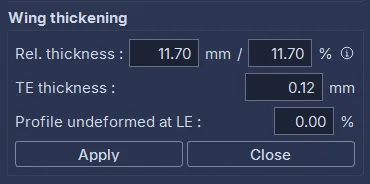
• Rel. thickness in mm and in %: the maximum thickness of the profile relative to the chord. Changing it scales the profile in thickness while keeping the camber line and the chord (the XFOIL method). The two fields are linked; the percentage is applied to both sides, each with its own chord.
• TE thickness in mm: opens (or closes) the trailing edge to the given thickness. The trailing edge is formed by the first and the last selected points: a profile closed to a point (first and last points coincident) opens too. A trailing edge closed to a point cannot be cut; 0.5 to 1 mm gives it a clean edge.
• Profile undeformed at LE in %: the part of the chord, from the leading edge, that keeps exactly the original profile; the opening of the trailing edge starts at this station and grows up to the trailing edge. At 0 %, the whole profile opens as a wedge from the leading edge. The value is used at the next validation of the trailing-edge thickness: to change it afterward, undo, then validate again.

Each validation of a field, or Apply, changes the project and counts as one undo step; the panel stays open, so that you can proceed in small steps. Close closes the panel.

For the relative thickness, the leading edge is the rightmost point (Xmax) and the trailing edge the leftmost point (Xmin); the two surfaces are separated by the chord. The selection must contain points of both surfaces.

4.13 Synchronizing side 1 / side 2

4.13.1 Principle

The wire passes through the points with the same number on both sides at the same time. Two paths can have the same number of points and still cut badly: if the points are distributed differently, the wire goes askew and the surface is distorted. The wire must pass through certain characteristic points at the same moment on both sides: the synchronization points.

4.13.2 Choosing the synchronization points

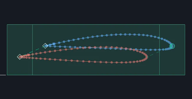
Switch to Sync. mode and click the points that must correspond, on both sides, in the lists or in the 3D view. For a wing, the leading edge (the rightmost point) is the first candidate. The first and the last points are always synchronization points, so there is no need to select them. Place as many as needed, always in pairs: the n-th point selected on side 1 corresponds to the n-th on side 2.

A dotted line joins each pair in the 3D view (visible in the image above, between the two leading edges), which lets you check the work when there are many pairs.

4.13.3 Applying the synchronization, synchronous cleanup

The Synchronization frame appears in Sync. mode. Click Synchronize: between each pair, the points of one side are projected onto the other at the same fraction of length, and vice versa. The two paths then have the same number of points, and the wire moves evenly.

Synchronization creates many points (50 points can become 97). The Synchronous cleanup after synchronization box, checked at first, immediately applies a synchronous cleanup with the tolerance of the Cleanup frame: a point is removed only if its counterpart can be removed too, and the synchronization points are always kept. This brings the number of points back down to a reasonable count (97 become 72) without losing the correspondence.

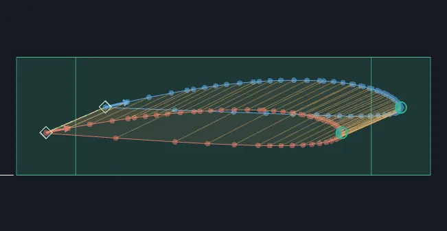
Three errors are reported: a different number of synchronization points on the two sides; fewer than two points on a path; two coincident synchronization points.

Synchronization is the essential step of complex cuts. Taking the time to do it properly guarantees the quality of the cut. Panels transferred from the Wing tab arrive already synchronized, with their synchronization points in place.

4.14 Stop points

A stop point is a point where the cut stops and waits for the operator to restart it: time to remove an offcut, or to wipe the wire. Stop points are placed when both sides have the same number of points, just before moving on to cutting.

Switch to Stops mode and click the point: its counterpart on the other side is selected automatically (stops always go in pairs). Each stop is marked by a pink ring on the path, in the Design 3D view (in every mode) as in the Cutting tab; during the cut, the wire stops on that very point, on a GRBL interface as on an IPL5X one, and the Resume button restarts the movement. The simulation of the Cutting tab stops there too.

The Cutting tab’s intermediate exits place their own stop points.

4.15 The intermediate profile

When a panel is wider than the machine’s table, it has to be cut in two. The Intermediate profile frame, under the point lists, computes the section of the panel at any distance from side 2, and splits the project into two documents at that distance.

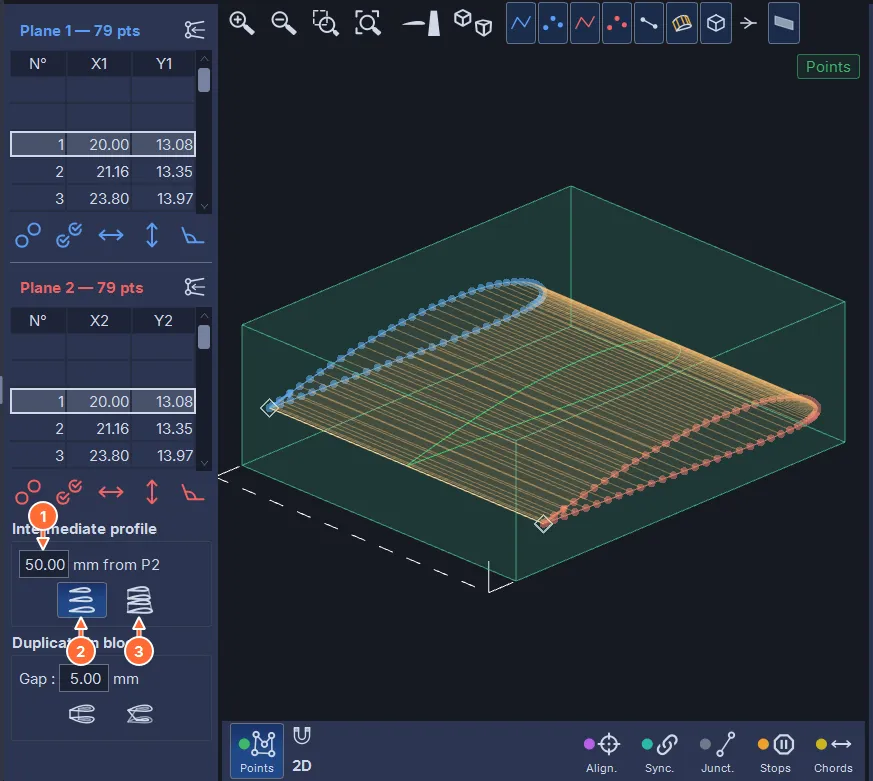
1. The distance, in millimeters from side 2.
2. Show: the intermediate profile appears in green in the 3D view. The distance can exceed the spacing, which extends the panel; it cannot be exactly 0 or the spacing.
3. The split button, whose tooltip reads “Split the project at the intermediate profile”: it creates two documents, one per half. It is active only while the green profile is shown, and the distance must be between 0 and the spacing.

The frame is grayed out when the two sides do not have the same number of points, or when the spacing is zero. The distance entered is kept; as soon as the project changes, the Show button pops back up: a click recomputes.

The split does not change the original document. It creates two free documents, named after it: ”… - P2 side”, from side 2 to the intermediate profile, and ”… - P1 side”, from the intermediate profile to side 1; the tab shows the first one. Both halves keep the same block bottom: the dihedral stays aligned at the joint, with nothing to note or to correct. The block margins in X are computed at the place of the split, so that a tapered wing keeps consistent margins on both sides of the joint. The joint faces are the side faces of the blocks, not wire cuts: dress each block to the length of its half.

The method for a 700 mm wing on a 560 mm table:

1. Define the wing at its final dimension (spacing 700) and save the project.
2. Enter the split distance, 400 mm for example, and click Show.
3. Click the split button: two documents appear in the chips, ”… - P2 side” (spacing 400) and ”… - P1 side” (spacing 300).
4. Cut each half: choose its chip, go to the Cutting tab, cut.
5. Glue the two pieces edge to edge.

The intermediate profile can also be exported as DAT or DXF with File ▸ Export ▸ Export intermediate profile…, at the distance entered.

4.16 Duplicate in block

When the block is thick enough, the two wings are cut from the same block. The Duplicate in block frame, under the intermediate profile, does this in one operation from the current panel. It is active when both sides have the same number of points.

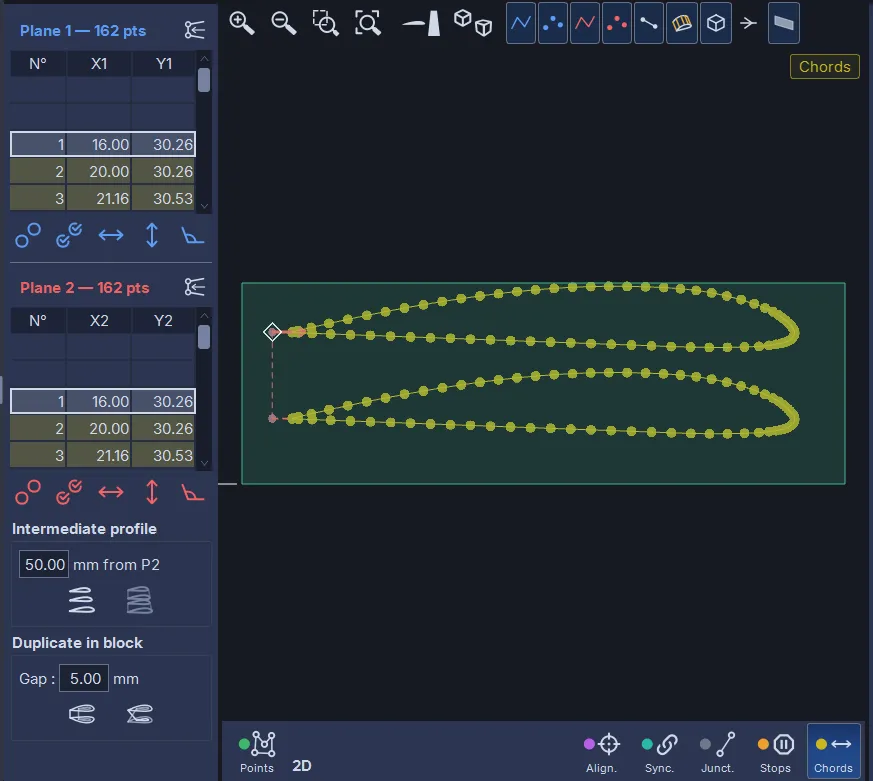
• Gap: the thickness of material left between the two cuts.
• The first button makes a mirror about a horizontal plane: the cut and its top/bottom mirror image in the same block. The bottom wing is traveled in the opposite direction to the top one.
• The second button makes a mirror about a vertical plane: the opposite wing (side 1 and side 2 swapped) is stacked under the original.

In both cases, the two cuts are connected by junction paths, with a 4 mm clearance at the trailing edge, and the number of points on each side doubles. The clearance segments add to the displayed chord; the profile points are marked in Chords mode, to which the tab switches at once to show them. The block is not resized: set its thickness afterward.

4.17 Background images

An image from the reference image bank (chapter 12) can be placed in a plane of the document, to scale, to trace a profile or to check it against a plan. It is a display aid, never a cut. Images are set up in the Images page of the right column, chosen with the tab at the bottom of the column.

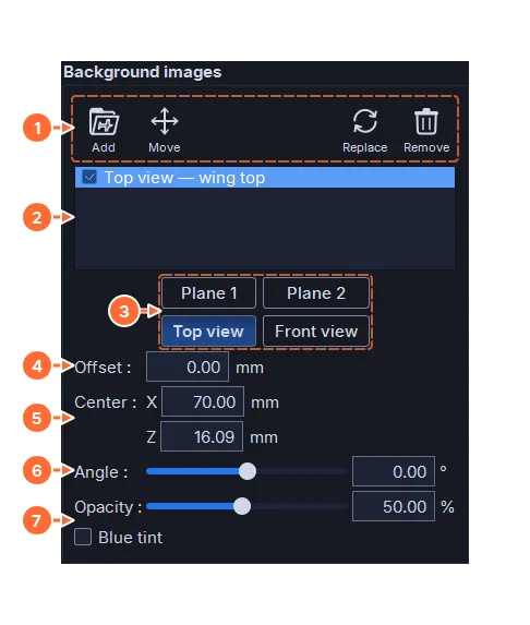
1. Add chooses an image from the bank and places it in Plane 1, centered on the side 1 profile; Move, Replace (another image from the bank in the same place, with the same settings) and Remove act on the selected image.
2. The list of the document’s images, named after their plane (“Plane 1 — wing top”), each with a display box; select a row to adjust it.
3. The plane of the image: Plane 1 and Plane 2, the cutting planes of the two sides; Top view, a horizontal plane; Front view, a vertical plane across the two sides, seen from the leading edge, to check a dihedral.
4. The offset: the height of a Top view image, the X position of a Front view image. It does not exist for Plane 1 and Plane 2.
5. The center of the image in its plane.
6. The angle, in degrees, positive counter-clockwise.
7. The opacity and the blue tint.

Move turns the view to face the image’s plane: you then drag the image with the mouse, and the mouse wheel zooms. Leaving the Images page, changing selection mode, taking the measuring tool or rotating the view (middle button, Alt + left button) ends the move.

The ninth display button of the 3D view, Background images, shows or hides all the images; each image’s box applies on top of that. The images are drawn behind everything else and do not count for View all.

The images belong to the document: they are saved with it, each addition, setting or move counts as one undo step, and changing document shows the other document’s images. Deleting an image from the bank removes it from all documents.

The images follow the project when the software realigns it in the block (after a change to the points, the block, Chords mode, the sweep or the dihedral): this realignment moves both sides together, and the images with them. On the other hand, the sweep, the dihedral and the alignment buttons move side 1 without its images: the drawings remain the reference on which these values are set, and side 2 always stays on its drawing. Likewise, a change to the points themselves (move, stretch, rotation, chord) moves the profile on the drawing without moving the image. An import into a side leaves the images in place.

The method for a wing: place a front view of the aircraft (or the two ribs on one drawing), fit it to the side 2 profile with Move, then adjust the sweep and the dihedral until side 1 meets its outline; the front view of the toolbar shows the dihedral against a Front view image.

Transfers from the Wing and Views tabs bring their images into the documents they create (chapters 8 and 10). The split at the intermediate profile gives the Plane 2 images to the “P2 side” half, the Plane 1 images to the “P1 side” half, and the Top view and Front view images to both.

4.18 The comment

The Comment button of the status bar opens a text area under the 3D view. The comment is saved in the project file; it is invaluable for noting the cutting conditions, the material or a kerf height, and for sharing a file. An imported path brings the comment of its source file, preceded by the side it was imported into.

4.19 Saving and exporting

• File ▸ Save (Ctrl+S) and Save As… write the .hw4x workspace.
• File ▸ Export ▸ Export Plane 1… or Export Plane 2… writes the path of one side as DAT or DXF (depending on the extension given); Export intermediate profile… exports the green profile at the distance entered. These entries are active only on the Design tab, and require an active license (chapter 16).
• A DAT is written like an ordinary wing profile: the leading edge at X = 0 and a chord of 1, with the same first point and the same direction of travel. It therefore does not keep the size: when imported again, it takes the chord of the side that receives it (100 mm on an empty side). To keep the millimeters, export as DXF.
• G-code export is done from the Cutting tab.